Introduction to Julia
![]()
The team (@github handles)
- Simone Silvestri (@simone-silvestri)
- fluid dynamicist with the passion of high performance computing
- developer of Oceananigans, ClimaOcean and ClimaSeaice
- Ludovic Raess (@luraess)
- computational geoscientist by day
- Julia GPU and HPC wizard the rest of the time (unless sleeping)
- Milan Kloewer (@milankl)
- 3
- 3
- Lazaro Alonso (@lazarusA)
- scientist by day, plotting wizard by night
- regular on Julia-discord, slack
- Mauro Werder (@mauro3)
- glaciologist by day
- programming Julia since 2013, maintainer of a few Julia packages
The format
Material is on GitHub https://github.com/mauro3/EGU2025-Julia-intro-and-showcase-for-geoscience
We try to make this short course a little interactive:
- either follow along with your local Julia & Jupyter install, or
- use Google Colab
to run (some of) the notebooks
In case someone doesn't know: Jupyter Notebooks
This is a Jupyter notebook; a browser-based computational notebook.
Code cells are executed by putting the cursor into the cell and hitting shift + enter. For more
info see the documentation.
The Julia programming language
Julia is a modern, interactive, and high performance programming language. It's a general purpose language with a bend on technical computing.
![]()
- first released in 2012
- reached version 1.0 in 2018
- current version 1.11 (04.2025)
- thriving community, for instance there are currently around 12000 packages registered
What does Julia look like
An example solving the Lorenz system of ODEs:
function lorenz(x)
    σ = 10
    β = 8/3
    ρ = 28
    [σ    * (x[2] - x[1]),
     x[1] * (ρ - x[3]) - x[2],
     x[1]*x[2] - β*x[3]]
end

# integrate dx/dt = lorenz(t,x) numerically for 500 steps
dt = 0.01
x₀ = [2.0, 0.0, 0.0]
out = zeros(3, 500)
out[:,1] = x₀
for i=2:size(out,2)
    out[:,i] = out[:,i-1] + lorenz(out[:,i-1]) * dt
end
And its solution plotted
using Plots # The plotting package may need to be installed with: using Pkg; Pkg.instantiate()
plot(out[1,:], out[2,:], out[3,:])
Julia in brief
Julia 1.0 released 2018, now at version 1.11
Features:
- general purpose language with a focus on technical computing
- dynamic language
- interactive development
- good performance on par with C & Fortran
- just-ahead-of-time compiled via LLVM
- No need to vectorise: for loops are fast
- multiple dispatch
- user-defined types are as fast and compact as built-ins
- Lisp-like macros and other metaprogramming facilities
- designed for parallelism and distributed computation
- good inter-op with other languages
The two language problem
One language to prototype -- one language for production
- example from a co-worker: prototype in Matlab, production in CUDA-C
One language for the users -- one language for under-the-hood
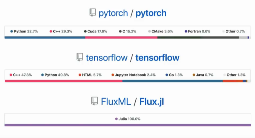
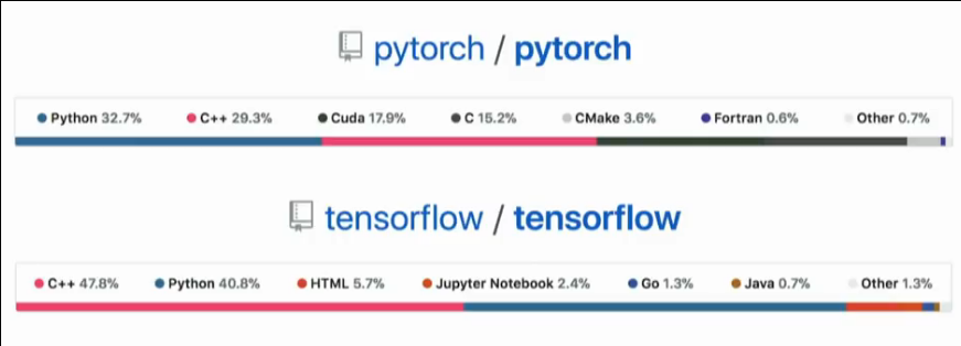
- Numpy (python -- C)
- machine-learning: pytorch, tensorflow
The two language problem
Prototype/interface language:
- easy to learn and use
- interactive
- productive
- --> but slow
- Examples: Python, Matlab, R, IDL...
Production/fast language:
- fast
- --> but complicated/verbose/not-interactive/etc
- Examples: C, C++, Fortran, Java...
Julia solves the two-language problem (mostly)
Julia is:
- easy to learn and use
- interactive
- productive
and also: fast