Worked Example: Unteraar Glacier

This page works through a complete subglacial routing analysis on Unteraar glacier, Switzerland, using the real bedrock and surface DEM data bundled with the package. It demonstrates the full WWFS → WWFR workflow:

deterministic subglacial routing with WhereTheWaterFlows.Subglacially, and
Monte Carlo uncertainty propagation over uncertain bed topography with WhereTheWaterFlows.Randomly.

Data source: Grab (2020), incorporating SwissTopo SwissALTI3D surface data (see References). Files are stored under examples/data/.

Loading the data

Unteraar glacier lies in the Bernese Oberland, Switzerland. The DEM covers a 539 × 459 grid of cells at 20 m spacing in the Swiss LV95 coordinate system.

using WhereTheWaterFlows, Statistics, CairoMakie
using Random; Random.seed!(42)

const WWFS = WhereTheWaterFlows.Subglacially
const WWFR = WhereTheWaterFlows.Randomly

datadir = joinpath(Base.pkgdir(WhereTheWaterFlows), "examples", "data")

nx, ny = 539, 459
beddem  = Matrix{Float32}(undef, nx, ny)
surfdem = Matrix{Float32}(undef, nx, ny)
x       = Vector{Float32}(undef, nx)
y       = Vector{Float32}(undef, ny)

open(joinpath(datadir, "bed.bin"),     "r") do f; read!(f, beddem);  end
open(joinpath(datadir, "surface.bin"), "r") do f; read!(f, surfdem); end
open(joinpath(datadir, "x.bin"),       "r") do f; read!(f, x);       end
open(joinpath(datadir, "y.bin"),       "r") do f; read!(f, y);       end

dx = x[2] - x[1]   # ≈ 20 m (LV95 easting spacing)
println("Grid: $(nx)×$(ny), dx = $(dx) m")

Grid: 539×459, dx = 20.0 m

The bed DEM has NaN everywhere outside the glacier (plotted white):

fig = Figure(size=(900, 340))
ax1 = Axis(fig[1,1]; aspect=1, xlabel="Easting (m)", ylabel="Northing (m)")
ax2 = Axis(fig[1,3]; aspect=1, xlabel="Easting (m)")
pl = heatmap!(ax1, x, y, surfdem; colormap=:viridis)
Colorbar(fig[1,2], pl, label="Surface elevation (m a.s.l.)")
pl = heatmap!(ax2, x, y, surfdem.-beddem;  colormap=:inferno)
Colorbar(fig[1,4], pl, label="Ice thickness (m)")
fig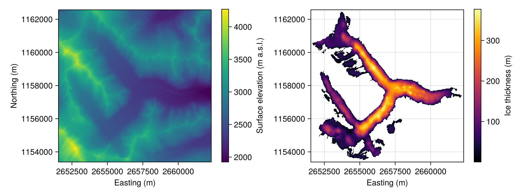

Preparing inputs

NaN bed values would propagate into the Shreve hydraulic potential φ = fH(ρᵢ/ρw) + zb, where H = zs − zb is ice thickness. We set the source to zero outside the glacier but route the water on the full DEM, i.e. it can leave the glacier.

# Replace NaN-bed cells with surface elevation (zero thickness → φ stays finite)
beddem_clean = copy(beddem)
glacier      = .!isnan.(beddem)
beddem_clean[.!glacier] .= surfdem[.!glacier]

# Uniform 1 cm/day melt source on glacier only, converted to m/s
source = fill(Float32(1e-2 / 86400), nx, ny)
source[.!glacier] .= 0

println("Ice-covered cells: $(sum(glacier)) / $(length(glacier)) ",
        "($(round(100*mean(glacier), digits=1)) %)")

Ice-covered cells: 56726 / 247401 (22.9 %)

Deterministic routing

waterflows_subglacial routes water according to the Shreve hydraulic potential, with optional Röthlisberger pressure-melting-point deflection controlled by gamma. Setting gamma = WWFS.GAMMA (≈ −0.31, the physical value) enables the full deflection model.

out = WWFS.waterflows_subglacial(
    surfdem, beddem_clean, dx,
    1.0,      # floatfrac: full flotation
    source   # basal melt source [m/s]
    ;
    gamma       = WWFS.GAMMA,
    drain_pits  = true,
    bnd_as_sink = true,
    nan_as_sink = true,
)

(; area, sinks, pits) = out.routing

println("Sinks (outlets):            ", length(sinks))
println("Unresolved pits:            ", length(pits))
println("Supercooled cells:          ", sum(out.pressmelt.sc_locs))
println("Max discharge [m³/s]:       ",
        round(maximum(area.total[glacier]), digits=4))
println("Max lake depth (fixed surf) [m water equivalent]:  ",
        round(maximum(out.lakes.depth_fixed_surface[glacier]), digits=1))
println("Max lake depth (free surface) [m]:   ",
        round(maximum(out.lakes.depth_free_surface[glacier]), digits=1))

Sinks (outlets):            1992
Unresolved pits:            0
Supercooled cells:          1255
Max discharge [m³/s]:       1.5801
Max lake depth (fixed surf) [m water equivalent]:  111.4
Max lake depth (free surface) [m]:   10.0

The flux can be visualised with the provided plotting function

plt_area(x, y, area.total; colorbar_label="log10(discharge (m3/s))")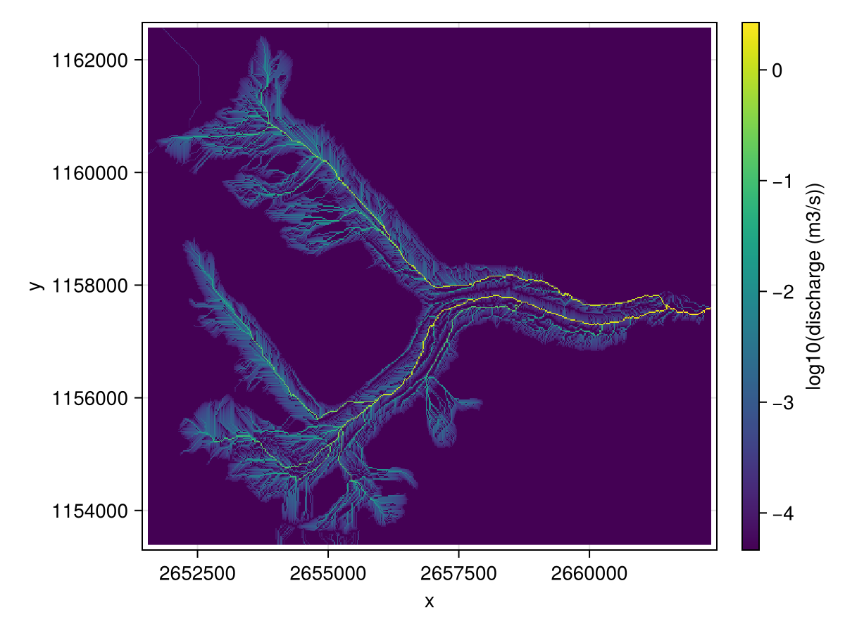

Interpreting the output:

Sinks are located on the domain boundary, thus streams leave the glacier area and flow through the periglacial region until they reach the domain boundary. There are no pits as they are all filled.
Supercooled cells arise where the bed slope opposing ice flow is steep enough for the Röthlisberger criterion to be met. With avoid_sc=false (default), water still routes through these cells; the physical interpretation is that R-channel flow is suppressed there but distributed flow continues.
Lake depths identify where subglacial water would pond before it can continue to flow downstream. But here less than 1% of the cells experience ponding.
Discharge units: area.total accumulates source × dx² (m³/s) plus dissipation- and pressure-melt contributions along each flow path.

Monte Carlo bed-uncertainty propagation

Bed topography beneath a glacier is derived from geophysical surveys and carries significant uncertainty. Here we propagate a 10 % relative bed uncertainty with a 100 m spatial correlation length through the routing model using the WWFR workflow:

Describe each uncertain field with WWFR.Uncertainty.
Build model, sample, and reduce! with WWFR.make_fns_subglacial.
Run the Monte Carlo loop with WWFR.map_mc.

# Surface treated as exact; bed carries 10 % relative uncertainty, 100 m corr. length,
# but only within the glacier boundary
surfdem_uc   = WWFR.Uncertainty()
beddem_uc    = WWFR.Uncertainty(reluc=0.1.*glacier,
                                correlation_length=100.0,
                                covariance_fn=WWFR.exponential_kernel)
floatfrac_uc = WWFR.Uncertainty()
source_uc    = WWFR.Uncertainty()

floatfrac_arr = fill(Float32(1.0), nx, ny)

model, sample, reduce! = WWFR.make_fns_subglacial(
    dx,
    surfdem,      surfdem_uc,
    beddem_clean, beddem_uc,
    floatfrac_arr, floatfrac_uc,
    source,       source_uc,
    [];                        # no explicit catchment-sink tracking here
    gamma = WWFS.GAMMA,
)

aggr = WWFR.map_mc(model, sample, reduce!, 10; progressmeter=false)

println("MC samples completed:        ", aggr.n_samples[])
println("Mean max discharge [m³/s]:   ",
        round(maximum(aggr.areas_total[glacier]), digits=4))
println("Max supercooling frequency:  ",
        round(maximum(aggr.sc_locs[glacier]),             digits=3))
println("Max lake-occurrence fraction:",
        round(maximum(aggr.lake_mask_fixed_surface[glacier]), digits=3))

MC samples completed:        10
Mean max discharge [m³/s]:   1.3326
Max supercooling frequency:  0.5
Max lake-occurrence fraction:1.0

Note

Ten samples is intentionally small for documentation build speed. For production use, 50–200 samples gives more stable statistics.

The mean flux can be visualised with the provided plotting function

plt_area(x, y, aggr.areas_total)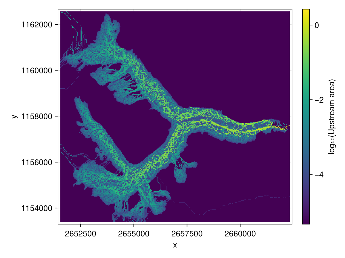

Interpreting the MC output

map_mc returns an aggregate named tuple with ensemble statistics:

For the full subglacial aggregate-output API (including shapes/types and reduction semantics), see the consolidated table in Randomly: Subglacial aggregate outputs.

Field	Contents
`aggr.areas_total`	Mean discharge field [m³/s] over all realizations
`aggr.sc_locs`	Fraction of realizations in which each cell was supercooled (0–1)
`aggr.lake_mask_fixed_surface`	Fraction of realizations with lake depth > 10 m (fixed-surface)
`aggr.lake_depth_fixed_surface`	Mean lake depth [m] over all realizations
`aggr.melt_rate`	Mean melt-rate field [m/s] over all realizations

A summary across all glacier cells:

sc_frac   = mean(aggr.sc_locs[glacier])
lake_frac = mean(aggr.lake_mask_fixed_surface[glacier])
println("Mean supercooling frequency (glacier cells): $(round(sc_frac,   sigdigits=3))")
println("Mean lake-occurrence fraction (glacier cells): $(round(lake_frac, sigdigits=3))")

Mean supercooling frequency (glacier cells): 0.0342
Mean lake-occurrence fraction (glacier cells): 0.18

Visualising results

Add CairoMakie to plot the spatial fields:

fig = Figure(size=(1100, 340))
ax1 = Axis(fig[1,1]; title="Mean discharge [m³/s]",
           xlabel="Easting (m)", ylabel="Northing (m)")
ax2 = Axis(fig[1,2]; title="Supercooling frequency",
           xlabel="Easting (m)")
ax3 = Axis(fig[1,3]; title="Lake-occurrence frequency",
           xlabel="Easting (m)")

heatmap!(ax1, x, y, log10.(aggr.areas_total);     colormap=:viridis)
heatmap!(ax2, x, y, aggr.sc_locs;                 colormap=:rain)
heatmap!(ax3, x, y, aggr.lake_mask_fixed_surface; colormap=:Blues)

fig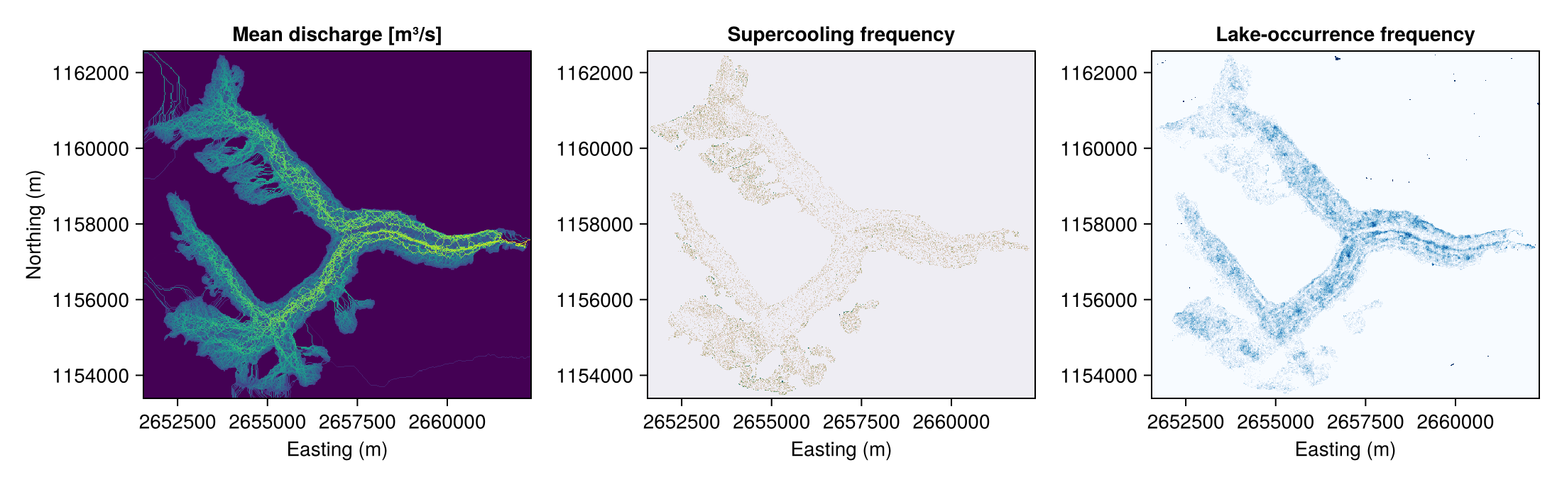

More examples can be found in the examples/ directory, see Example scripts.