WhereTheWaterFlows.Randomly (WWFR)

WWFR provides Monte Carlo wrappers to propagate field uncertainty through deterministic routing models.

It supports subaerial routing uncertainty (make_fns_subaerial), subglacial routing uncertainty (make_fns_subglacial). It implements the spatial uncertainty in the input fields using configurable Gaussian random fields (GRFs) which produce spatially correlated noise.

Workflow

Typical usage is:

1. define uncertainty models for uncertain fields,
2. build model, sample, and reduce! with make_fns_*,
3. run Monte Carlo with map_mc.

The key design idea is that map_mc is generic: it does not know anything about routing fields. It only calls three functions you provide:

• sample(): generate one stochastic input realization,
• model(args...): run one deterministic forward model,
• reduce!: aggregate outputs over many realizations.

Uncertainty model

Uncertainty stores how one field should be perturbed:

Uncertainty(; absuc=0,
              reluc=0,
              correlation_length=1,
              covariance_fn=gaussian_kernel,
              abs_bounds=(-Inf, Inf))

For a base field f, each realization is generated as:

1. draw a zero-mean unit-variance correlated GRF xi,
2. scale it with absolute and relative amplitudes,
3. optionally clip perturbation values,
4. add perturbation back to the field.

In code terms (as implemented):

delta = xi .* absuc .+ xi .* f .* reluc
delta = clamp.(delta, abs_bounds...)
f_realization = f .+ delta

Parameter meaning

GRFs: how they work

WWFR uses FFT-based GRF sampling (following Raess et al., 2019).

Correlation length conversion: if the grid spacing is dx, then WWFR converts:

len = correlation_length / dx

so kernels operate in cell units.

Kernel choice:

• gaussian_kernel: smoother, more diffuse perturbations
• exponential_kernel: rougher, shorter-scale structure for same nominal length
• custom kernel: pass any kernel_fn(nx, ny, len) compatible function

What can be configured

High-level Monte Carlo controls:

• map_mc(model, sample, reduce!, n; progressmeter=true)
• n: number of realizations (n <= 2048 enforced)
• progressmeter: set false for quiet batch/CI runs

Subaerial wrapper (make_fns_subaerial):

• uncertain fields: dem, source
• routing controls: drain_pits, bnd_as_sink, nan_as_sink
• sink groups for aggregation: ctch_sinks

Subglacial wrapper (make_fns_subglacial):

• uncertain fields: surfdem, beddem, floatfrac, source
  • Note: unlike waterflows_subglacial, which accepts scalar floatfrac, make_fns_subglacial requires floatfrac to be an array.
• physical controls: gamma, rhow, rhoi
• processing controls: mask, ctch_sinks, min_lake_depth

Why reduction is needed

A Monte Carlo run can easily produce hundreds of large 2D outputs. Storing all realizations is expensive and often unnecessary. reduce! keeps only summary statistics (means, frequencies, selected per-sample vectors), which is both memory-efficient and directly useful for interpretation.

In WWFR wrappers, reduction happens in three stages:

1. reduce!() initializes aggregate storage.
2. reduce!(aggr, sample_output) updates aggregate values per realization.
3. reduce!(aggr) finalizes (typically divides accumulated maps by n).

How outputs are reduced

Subaerial

The reduction function returned by make_fns_subaerial accumulates:

• areas_total += output.area
• stream_length += output.slen
• catchments[:, :, i] += catchment(output.dir, ctch_sinks[i])
• catchment_fluxes[i] stores one scalar per sample (not averaged in place)

At the finalize step map-style fields are normalized by n_samples (so they are means/frequencies) and flux vectors remain per-sample records by design.

Subglacial

The reduction function returned by make_fns_subglacial accumulates: routed maps and diagnostics (areas_total, lake_depth_*, lake_mask_*, sc_locs, kappas, catchments) and appends sink-flux records to vectors (catchment_fluxes.total/dissipation/pressmelt).

At the finalize step map-style fields are normalized by n_samples (so they are means/frequencies) and flux vectors remain per-sample records by design.

When ctch_sinks is non-empty, aggr.catchment_fluxes has subglacial-specific structure:

• aggr.catchment_fluxes is a named tuple (total, dissipation, pressmelt).
• Each field is a Vector with length length(ctch_sinks).
• Element i of each field is a Vector{Float32} with length n_samples, containing the per-realization flux for outlet group i.

So for subglacial runs, the total-flux distribution at outlet group i is accessed as aggr.catchment_fluxes.total[i]. This differs from the subaerial wrapper, where per-outlet total fluxes are stored directly as aggr.catchment_fluxes[i] (no .total).

Minimal usage pattern:

using Statistics

for i in eachindex(ctch_sinks)
    fluxes = aggr.catchment_fluxes.total[i]   # Vector{Float32}, length n_samples
    println("Outlet $i: mean=$(mean(fluxes)), std=$(std(fluxes))")
end

ctch_sinks: what it means

ctch_sinks defines sink groups, as described in Subglacially: Defining outlet groups, for which WWFR reports catchment membership and integrated fluxes.

Each element of ctch_sinks is a collection of sink cells (typically a Vector{CartesianIndex} or CartesianIndices). For each Monte Carlo sample, WWFR computes the full upstream catchment draining to each sink group. You can pass multiple groups, e.g. upper/lower terminus sectors, to compare how uncertainty redistributes flux between outlets.

This enables statistics like:

• probability that a cell drains to outlet group i (aggr.catchments[:, :, i]),
• distribution of total flux entering outlet group i (aggr.catchment_fluxes[i] in subaerial, and aggr.catchment_fluxes.total[i] in subglacial).

Defining custom make_fns_*

The built-in make_fns_subaerial/make_fns_subglacial are templates. If your model has different outputs, constraints, or diagnostics, define your own trio:

• model(args...)
• sample()
• reduce! (three-method interface)

then call map_mc(model, sample, reduce!, n).

Minimal skeleton:

model(a, b) = my_forward_model(a, b)
sample() = (draw_a(), draw_b())

function reduce!()
    return (sumfield = 0.0, n = Ref(0))
end

function reduce!(aggr, out)
    aggr.sumfield += out.metric
    aggr.n[] += 1
    return aggr
end

function reduce!(aggr)
    aggr.sumfield /= aggr.n[]
    return aggr
end

The reduce! function has three methods: 0-arg method sets up the storage needed in the reduction (this gets called once at the beginning of the mc-iterations); the 2-arg method is called after each forward model evaluation and reduces/aggregates the forward model output into what is stored; the 1-arg method is then called at the end to finalize the aggregated results.

Note: only reduce! is allowed to not be thread-safe, model and sample need to be thread-safe.

Minimal subaerial example

using WhereTheWaterFlows, CairoMakie
using Statistics
using Random; Random.seed!(42)

WWFR = WhereTheWaterFlows.Randomly

n = 80
dx = 100.0
x = range(-pi, pi, length=n)
dem = sin.(x) .* cos.(x')
source = fill(1e-3 / dx^2, size(dem))

dem_uc = WWFR.Uncertainty()  # fixed DEM
source_uc = WWFR.Uncertainty(absuc=0.0, reluc=0.2, correlation_length=15 * dx)

ctch_sinks = [CartesianIndices((1:n, 1:1))[:]]

model, sample, reduce! = WWFR.make_fns_subaerial(dx,
                                                 dem, dem_uc,
                                                 source, source_uc,
                                                 ctch_sinks)

aggr = WWFR.map_mc(model, sample, reduce!, 100; progressmeter=false)

mu, sd = mean(aggr.catchment_fluxes[1]), std(aggr.catchment_fluxes[1])
hist(aggr.catchment_fluxes[1],
     axis=(title  = "mean = $(round(mu, sigdigits=4)), std = $(round(sd, sigdigits=4))",
     xlabel = "flux", ylabel="freq."))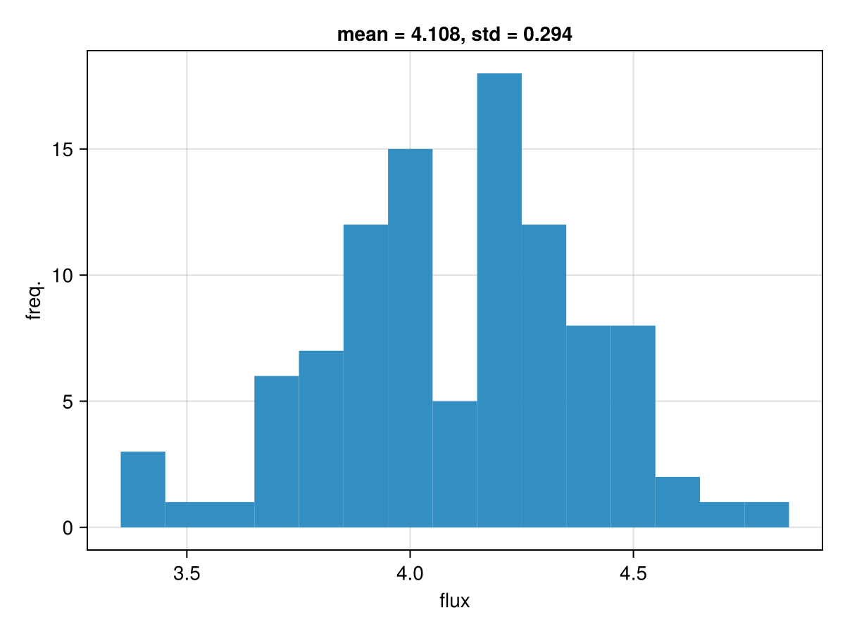

Output interpretation

Subareal aggregate outputs (make_fns_subaerial)

For subaerial runs, aggregated outputs:

• areas_total: Monte Carlo mean routed area/discharge field
• stream_length: Monte Carlo mean stream-length field
• catchments: per-sink occurrence frequency map (0-1)
• catchment_fluxes: per-sink vectors of sample fluxes

Subglacial aggregate outputs (make_fns_subglacial)

The table below consolidates all fields produced by aggr = map_mc(...) when using make_fns_subglacial.

Notes:

• For aggr.catchment_fluxes.*, element i is the flux distribution for outlet group i; each inner vector has length aggr.n_samples.
• If ctch_sinks is empty, aggr.catchments has zero groups and aggr.catchment_fluxes.* are empty vectors.

Practical guidance

• Use absuc for additive error floors; reluc for proportional uncertainty.
• Keep correlation_length meaningfully smaller than domain size (as a rule of thumb, at least around 3x smaller than domain extent).
• Set Random.seed! before building samplers for reproducible runs.
• Start with small n while validating model setup; scale up after checks.

Examples

• examples/wwfr-simple.jl: quick start
• examples/randomly/source-uncertainty-sweep.jl: source-vs-DEM uncertainty comparison and sensitivity sweep
• examples/subglacially/ice-cap-full-workflow.jl: subglacial deterministic+ Monte Carlo workflow, including sink discovery and ctch_sinks partitioning for per-outlet flux distributions

From the examples/ environment:

include("wwfr-simple.jl")
include("randomly/source-uncertainty-sweep.jl")
include("subglacially/ice-cap-full-workflow.jl")

See also: Examples, Subglacially, and API Reference.